Image Segmentation
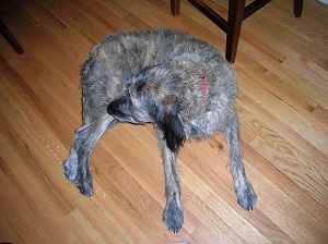
Jed Chou and Anna Weigandt The image segmentation problem is the following: given an image, a vector of pixels each with three associated red, green, and blue (RGB) values, determine which pixels should belong to the background and which should belong to the foreground. For example, in the following picture, the pixels which make up the dog should belong to the foreground, and the pixels making up the wood planks should belong to the background.
Summary
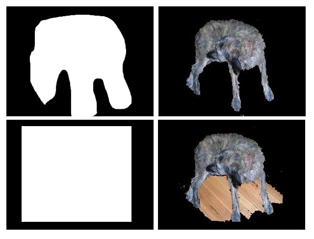
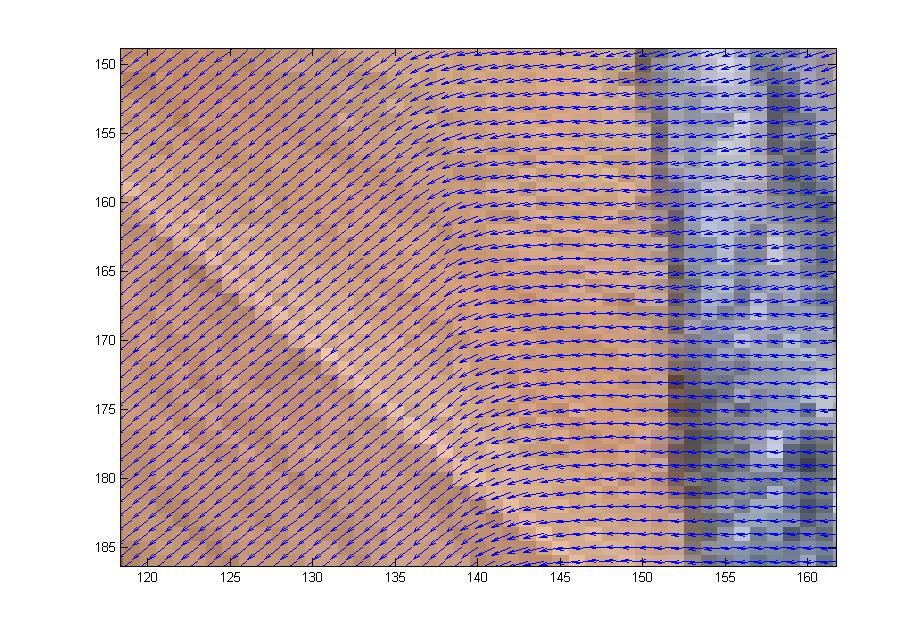
First we studied the grabCut algorithm and some general theory of image segmentation; we also played with some implementations of the grabCut algorithm to get a feel for how it worked. Anna wrote her own implementation of grabCut in matlab based on Gaussian Mixture Models which would take as input an image along with a manually-drawn matte and spit out a segmentation of the image into foreground and background. Our first goal was to get a clean segmentation of the dog picture shown above. Over the weeks we experimented with the dog picture by adjusting the algorithm parameters and we also discussed ways to extract more information from the color data to enhance the performance of Anna’s implementation. We added several matlab functions to do this. In the dog picture above, the problem mostly seemed to be that cutting along the long, upside-down U-shape between the dog’s hind legs and front legs was more expensive than cutting along the shorter distance spanned by a straight line from the bottom of the hind legs to the bottom of the front legs. We suspected that we needed to make it easier to cut along the this upside-down U-shape by decreasing the neighborhood weights along that arc. However, it wasn’t enough to just manually adjust the neighborhood weights–we wanted a way to automatically adjust the neighborhood weights so that such problems wouldn’t occur for other images. So our problem was to figure out which neighborhood weights to adjust and how to adjust them. First we tried using the directionality of the color data. The intuition was that if the colors in a subset of the image were running along a particular direction, then there should be an edge along that direction in the subset of pixels. We tried to capture the directionality in the color data by calculating the covariance matrix over small square windows of the image (the variance-covariance matrix of the variables X and Y where X was a vector consisting of the differences in color intensity in the horizontal direction and Y was a vector consisting of the differences in color intensity in the vertical direction). We then computed the spectrum of the covariance matrix centered at each pixel in the image. If the absolute value of the largest eigenvalue of the matrix was much greater than the absolute value of the smaller eigenvalue (which indicates a strong directionality along the direction of the corresponding eigenvector in that particular window), and also the largest eigenvector was almost horizontal or almost vertical, then we would decrease the corresponding horizontal or vertical neighborhood weight proportionally to the ratio of the eigenvalues. In theory this would make it less expensive to cut along the edges in the image. To check if the code was picking up directionality properly, we placed a vector field over the image where the vector at a pixel p was the eigenvector of the largest eigenvalue of the covariance matrix centered at p. Though the vector field seemed to capture the directionality properly, tweaking the edge weights in this way seemed to have little effect on the output of the algorithm: the large piece of wood flooring between the dog’s legs was still being categorized as foreground, even after we greatly magnified the adjustments to the edge weights based on the ratio of eigenvalues.
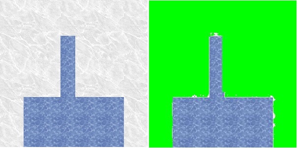
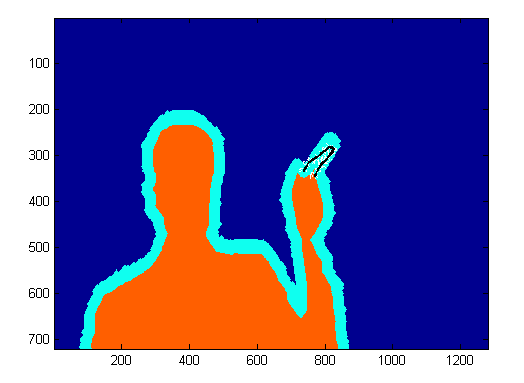
We next experimented with modifiying select node and neighborhood weights on the finger image. We manually marked certain pixels of the finger of the test image and adjusted the weights so that the selected pixels were forced into the foreground. This strategy only ensured the selected pixels were placed in the foreground. It failed to pull the rest of the finger into the foreground.