Category Archives: internships

2016 summer program

by

Computational Mathematics Bootcamp

Tuesday June 7 – Saturday June 18 (no meetings on Sat-Sun June 11-12)
Location: 239 Altgeld Hall
Instructor: Anil Hirani.

More information is here.

Prepare and Train
Monday June 20 – Friday July 29
Location: 159 Altgeld Hall
Instructor: Maxim Arnold (U of Texas at Dallas), assisted by Yuliy Baryshnikov (U of Illinois at Urbana-Champaign)

The program is a “Research Experience for Graduate Students” style endeavor: after a series of introductory lectures, the students form small groups (2-5 people) to work on open-ended interconnected problems.

This year the overall theme is Topologically constrained problems of statistical physics.

The goal is to guide students through the transition from working on “canned” problems to tackling open-ended problems and formulating the problems themselves. We expect the group work to involve a mixture of computational experiments (to generate conjectures) and theory (to prove them).

More information is here.

Workshop in Linear Algebra

Monday June 6 – Thursday July 28 (no meetings July 4-8)
Times: 5:30-7:00pm on Mondays and Thursdays
Location: 145 and 159 Altgeld Hall
Instructor: Derek Jung

Each session will begin with a 40-45 minute lecture. Then after a break, participants will work together on a problem set for 40-45 minutes. No work is expected outside of class.

Prerequisites: some linear algebra and proof techniques from prior math courses, along with enthusiasm and willingness to work with others. All undergraduate and graduate students are welcome to participate, whether or not you are involved in the other PI4 activities.

More information is here.

Internships

Various dates. Hosts to be arranged. Companies and faculty members interested in mentoring a student in this program, please register here.

Application procedure

Students: click here to apply to PI4 for Summer 2016.

2015 summer program

by

The summer program kicks off with the two week Bootcamp:

Computational Mathematics Bootcamp
Tuesday May 26 – Friday June 5
Location: 239 Altgeld Hall
Instructor: Sean Shahkarami
Coordinator: Anil Hirani

Prepare and Train
Monday June 15 – Monday July 27
Location: 159 and 173 Altgeld Hall
Instructor: Boris Shapiro, Univ. of Stockholm
Topics: Random matrix pencils, their related sorting networks, monodromy, and applications to physics. Students will explore open problems using theoretical and computational methods – the problems will cover several levels of difficulty, and so both beginning students (“Prepare”) and continuing students (“Train”) are welcome. The mathematical methods will be drawn from linear algebra, spectral theory, probability, geometry, and complex analysis.

Internships

Various dates. Hosts to be arranged.

Those interested in mentoring a student in this program, please register at https://illinois.edu/fb/sec/5413644

Internship at Personify: How to Stand out in a Picture

by

Image Segmentation

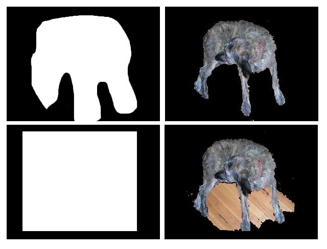
Jed Chou and Anna Weigandt The image segmentation problem is the following: given an image, a vector of pixels each with three associated red, green, and blue (RGB) values, determine which pixels should belong to the background and which should belong to the foreground. For example, in the following picture, the pixels which make up the dog should belong to the foreground, and the pixels making up the wood planks should belong to the background.

maggie
In 2004 Rother, Kolmogorov, and Blake introduced one solution to the image segmentation problem, an algorithm called GrabCut. Roughly, GrabCut works by forming a weighted graph from the pixels, defining an energy or cost function from this graph, and then finding a cut of the graph (an image segmentation) which minimizes the energy function. This minimum cut should in theory yield a good demarcation between background and foreground. We describe the steps in more detail below: First the user specifies an initial segmentation by drawing a rectangle on the image. Everything outside the rectangle is labelled “background” and the pixels inside are labelled “unknown”. Later the user may also mark certain pixels as foreground. A partition of the pixels into three components, foreground, background, and unknown, is called a trimap. Using this initial segmentation, GrabCut creates two Gaussian mixture models (GMMs), one for the background and one for the unknown. A graph is then formed with one node for each pixel and a set of edges connecting neighboring pixels. Each node is assigned a weight based on the GMMs. Each edge, say the edge between node A and node B, is assigned a weight based on the difference between the color intensities at A and at B. An energy function is defined: E=U+V, where U depends on the node weights and V depends on the edge weights. Some algorithm, such as MaxFlow or MinCut, is used to compute the minimum. The minimum energy state should correspond to a good segmentation. GrabCut works very well for many images, but it is sensitive to the initial trimap. In the pictures below, two different trimaps of the same image yield very different results.

mat
In one case, a rectangle is drawn around the dog and in the other, a more detailed outline of the dog is specified. For this image, a simple rectangle around the dog doesn’t provide GrabCut enough information to find a good segmentation. GrabCut, as it was first introduced, does not allow the user to draw a non-rectangular shape for the initial trimap, but it can fix the type of problem shown above by taking additional user input. Our task is to modify GrabCut so that it makes good cuts automatically in such cases, without requiring any additional input beyond the initial rectangular trimap.

Summary

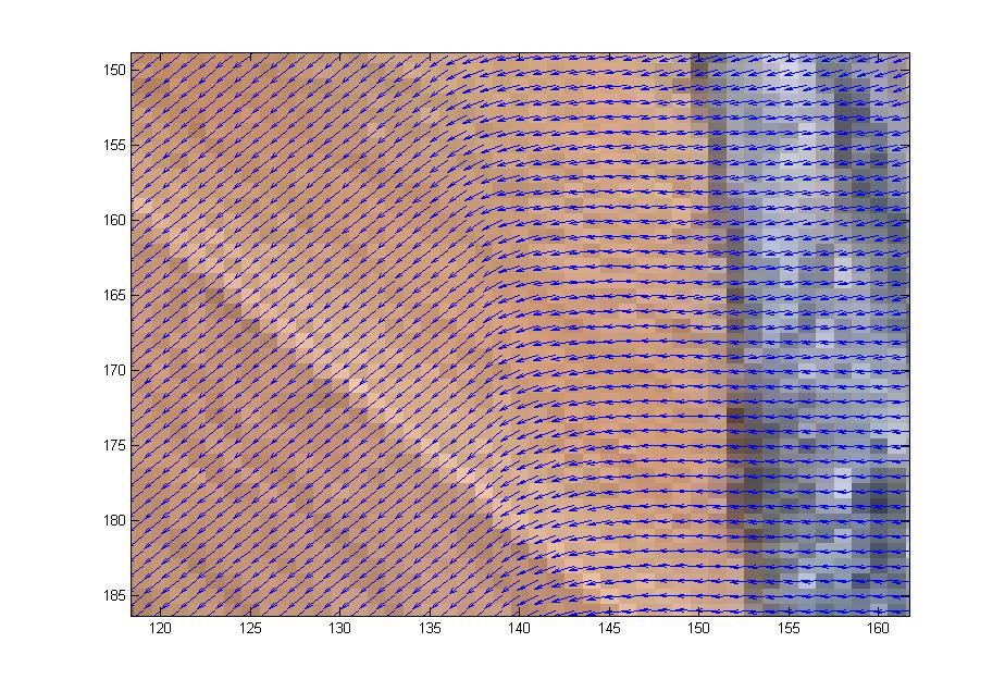
First we studied the grabCut algorithm and some general theory of image segmentation; we also played with some implementations of the grabCut algorithm to get a feel for how it worked. Anna wrote her own implementation of grabCut in matlab based on Gaussian Mixture Models which would take as input an image along with a manually-drawn matte and spit out a segmentation of the image into foreground and background. Our first goal was to get a clean segmentation of the dog picture shown above. Over the weeks we experimented with the dog picture by adjusting the algorithm parameters and we also discussed ways to extract more information from the color data to enhance the performance of Anna’s implementation. We added several matlab functions to do this. In the dog picture above, the problem mostly seemed to be that cutting along the long, upside-down U-shape between the dog’s hind legs and front legs was more expensive than cutting along the shorter distance spanned by a straight line from the bottom of the hind legs to the bottom of the front legs. We suspected that we needed to make it easier to cut along the this upside-down U-shape by decreasing the neighborhood weights along that arc. However, it wasn’t enough to just manually adjust the neighborhood weights–we wanted a way to automatically adjust the neighborhood weights so that such problems wouldn’t occur for other images. So our problem was to figure out which neighborhood weights to adjust and how to adjust them. First we tried using the directionality of the color data. The intuition was that if the colors in a subset of the image were running along a particular direction, then there should be an edge along that direction in the subset of pixels. We tried to capture the directionality in the color data by calculating the covariance matrix over small square windows of the image (the variance-covariance matrix of the variables X and Y where X was a vector consisting of the differences in color intensity in the horizontal direction and Y was a vector consisting of the differences in color intensity in the vertical direction). We then computed the spectrum of the covariance matrix centered at each pixel in the image. If the absolute value of the largest eigenvalue of the matrix was much greater than the absolute value of the smaller eigenvalue (which indicates a strong directionality along the direction of the corresponding eigenvector in that particular window), and also the largest eigenvector was almost horizontal or almost vertical, then we would decrease the corresponding horizontal or vertical neighborhood weight proportionally to the ratio of the eigenvalues. In theory this would make it less expensive to cut along the edges in the image. To check if the code was picking up directionality properly, we placed a vector field over the image where the vector at a pixel p was the eigenvector of the largest eigenvalue of the covariance matrix centered at p. Though the vector field seemed to capture the directionality properly, tweaking the edge weights in this way seemed to have little effect on the output of the algorithm: the large piece of wood flooring between the dog’s legs was still being categorized as foreground, even after we greatly magnified the adjustments to the edge weights based on the ratio of eigenvalues.

directionality
We then examined the the average node weight and the average neighborhood weight and found that the neighborhood weights were about 10^-5 times smaller than the node weights. This led us to think about adjusting the node weights instead. When we changed the number of components in our Gaussian mixture model to one instead of five, we obtained a clean segmentation of the dog from the background as shown below. For images in which colors are relatively uniform, this approach probably works well. Next we examined a sequence of images from Personify in which a person’s finger was improperly assigned to the background. The problem was similar to the one we encountered for the dog picture: it was too expensive to cut along the outline of the finger rather than across it. We tried ajusting the number of Gaussian components to no avail, so again we tweaked the edge weights.

blocktest
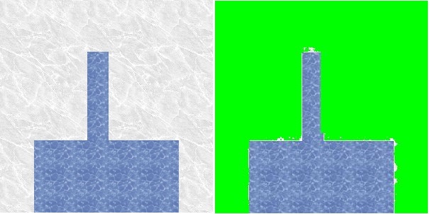
To attempt simplify the problem, we created noisy images of two rectangles sitting atop each other as shown above. However, the set of test images was not reflective of the finger situation. Given a trimap designating the upper rectangle as unknown, grabcut segmented the foreground from the background for all test images.

We next experimented with modifiying select node and neighborhood weights on the finger image. We manually marked certain pixels of the finger of the test image and adjusted the weights so that the selected pixels were forced into the foreground. This strategy only ensured the selected pixels were placed in the foreground. It failed to pull the rest of the finger into the foreground.

trimap
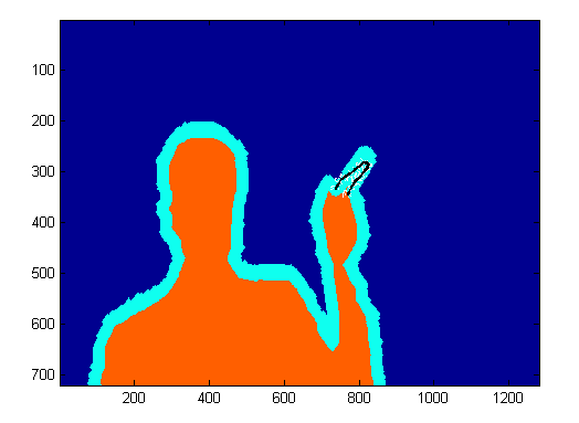
The second strategy seems more promising. We marked a band of pixels around the finger. We then adjusted those pixels by multiplying by some constant, c. Very low values of c, around the order of c=.01, ensured the finger was pulled into the foreground. Marking fewer pixels, near the end of the finger, sometimes was effective, but often would result in portions of the finger being lost. The current direction of work is to experiment with the selection of marked pixels.

Summer reports: working with applied mathematicians on real life problems

by

Several of our interns spent the summer working on various mathematical models stemming from real life challenges: understanding stability in power networks in their postmodern complexity; disentangling the intricacies of online search on two lines and understanding the limb development.

Below are their reports:

Nicholas Kosar, supervised by Alejandro Dominguez-Garcia;

Argen West, supervised by Prof. Zharnitsky;

Daniel Carmody and Elizabeth Field, supervised by Prof. Rapti;

Ben Fulan, supervised by Prof. Ferguson.

summer reports: shaping the canopy

by

PI4 Interns Nuoya Wang and Matthew Ellis spent this summer doing research under direction of Dr. Lebauer, a Research Scientist at Photosynthesis and Athmospheric Change Lab of UofI’s Energy Biosciences Institute. Below is their report.

This summer we focused on building a sugarcane canopy model and investigating into the direct sunlight photosynthesis effect.

The first task is how to extract features from a 3D image of one canopy. The data format is triangular mesh, which means the leaves and stems are divided into little triangles. This gives us a clue that we may use neighborhood relationship to define the structure of the canopy.

Firstly, it is easy to find the height of the canopy. We just need to find the points with largest z-coordinate and smallest z-coordinate then the difference is the height. So the main task is to extract leaf length, leaf width and leaf curvature.

To obtain features of a leaf, we need to divide a plant into different leaves and analyze each leaf. Since the plant is represented by a triangular mesh, we can interpret it into a graph. That is, we find unique vertices and construct the adjacency matrix. For example, if there are 10,000 unique points, our adjacency matrix will be a 10,000×10,000 one and if 10, 100, 1000 form a triangle, then the (10, 100), (100, 10), (10, 1000), (1000, 10), (100, 1000), (1000, 100) elements in matrix will be marked as 1.

We can use connected components algorithm, say, Bellman-Ford algorithm to split the graph into isolated components. In our sample data, it is more direct to do this because each leaf is not really “attached” to the stem which means stem is isolated from leaves. If the data is from reconstruction of real world data, we need to clean the data first, for example, we can calculate the number of neighbors for each vertex and delete some vertices with few neighbors. In this way some attached points will be separated. In the following figure 1, we have marked different components by different colors.

Since we have got one leaf from previous step, we can start to analyze it. The algorithm we use is Minimum Spanning Tree Algorithm.

In our problem we choose “weight” as the Euclidean distance between different points. After applying minimum spanning tree algorithm some of the unimportant connections are ignored and result is in figure 2:

Left: Figure 1; Right: Figure 2.

It is clear in figure 2 that the path which connect 2 red points can be used to estimate leaf length. So we used shortest path algorithm to find the path and calculate the path length. The 2 red points are defined as the pair with longest Euclidean distance. Leaf width can also be calculated from this minimum spanning tree. My algorithm is checking all points on the shortest path which connects the 2 red points, find 2 closest neighbors and leaf width at that point is defined as the sum of distance from the 2 neighbors. Finally, we choose the largest width as the width for whole leaf. Once we have the Euclidean distance of the 2 red points and the length of path connecting them, we can easily find the leaf curvature.

The second task in the summer project is to discuss the photosynthesis effect. We only considered the effect of direct sunlight. Our goal is to find the relationship between sunlit area ratio and height. The canopy model we used is still the triangular mesh model we have mentioned above.

In this part we focus on all vertices and introduce randomness into our algorithm. The basic principle for the algorithm is very simple: first we group all triangles’ vertices according to their heights. Second step is randomly choosing some points in one layer (that is, one group) to check if those points are shaded by higher level points or not. For example, if there are 1000 points in that group in total and we choose 200 of them. After calculation there are 100 points being shaded, then we assume there are 500 points being shaded in the original group. Using this simple sampling method, we can improve the efficiency of our algorithm by a lot.

Following are the results for direct sunlit ratios. In figure 3, x-axis is the height and y-axis is the ratio of shaded area. We tried several sunlight angles and got different results.

Figures 3 and 4 show the results. In figure 3, the azimuth angles for 3 pictures are 30, 60 and 90 degrees. Black lines are elevation=30 results, blue lines are for elevation=60 and red lines are for elevation=90. In figure 4, elevation angles for 3 pictures are 30, 60 and 90 degrees. Magneta lines are azimuth=0 results while black lines are azimuth=30 results, blue lines are for azimuth=60 and red lines are for azimuth =90.

internships: Ferguson’s lab

by

Ben Fulan worked on this project at Andrew Ferguson’s lab.

 Here’s  Ben’s final report.

This project arose out of the search for a vaccine to combat HIV and the obstacles faced by this search. While it is possible to create a vaccine that induces an immune response against the virus, the effectiveness of this approach is limited by the ability of the virus to mutate into strains which would no longer be targeted by the immune response. The goal of this project is to produce an immune targeting scheme that can do the most damage to the virus while taking into account its ability to mutate.

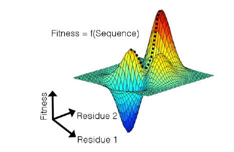
To this end, a measure of the fitness of the virus is needed. This takes the form of a fitness landscape, which gives the virus’s ability to replicate as a function of its amino acid sequence. (See figure below – the dashed line indicates a mutation path from a potentially immune-targeted global maximum to a local maximum.) In particular, this amino acid sequence can be described using a binary string, where 0 represents the natural (“wild type”) form of the amino acid and 1 represents a mutant. The fitness function can then be constructed from empirical data. This function assigns a fitness cost to each mutation and also contains terms to represent interactions between pairs of mutations, which can be either beneficial or harmful.

Once we have obtained the fitness function, we can add a term representing immune pressure that, for each amino acid, imposes a penalty for not mutating, effectively forcing the virus to mutate into a lower-fitness state. This modified function measures the viral fitness given a particular amino acid sequence; the next step is to produce a function that measures the overall fitness of the virus across all possible states. This function should give more weight to high-fitness states, since it is more likely that the virus will be found in such a state. One such function is
\[
\sum_z \exp{−\beta E(z,b)},
\]
where \(E\) is a version of the fitness function described above (in this case low energy corresponds to high fitness), \(z\) is the binary amino acid sequence, \(b\) is the sequence representing immune pressure, and the “inverse temperature” \(\beta\) represents the difficulty of mutation. Finally, we can cast the problem as an optimization problem as follows: minimize the overall fitness function subject to constraints on b (since only so much immune pressure can be applied). We then develop an algorithm to perform this optimization and obtain an optimum immune pressure sequence \(b\).

FitnessLandscape

We can then check these results against empirical data; if the data match poorly, we can reconsider our choice of the overall fitness function.

internships: at John Deere

by

We will start a series of posts about the topics our interns are working on. We start with Sishen Zhou and Han Wang, who are working this summer at John Deere, dealing with

Data Analysis for High Precision Agriculture

Maps of yield distribution are crucial for precision agriculture. A yield map with high resolution can help farmers precisely perform future agricultural operations, such as applying fertilizer and planting seeds according to geographic data.

The problem we are working on at John Deere is to find a way to determine the response function of a combine harvester that mixes plants during the harvest operation.

2023b

To be more precise, the crop cut from the field takes a while and multiple paths within the combine from cutting to measurement at the crop yield monitor. This delay and mixing is captured in a response function, and the readings of the yield monitor is approximately a convolution of the real yield distribution with the response function. So once we find the response function, we will be able to create a much more accurate map of yield distribution with deconvolution algorithms.

The following figure illustrates a response function and the delay caused by it at the yield monitor readings.

figure

This problem is not trivial since the yield is processed within the combine in several complicated steps. The combine has to be treated as a black box causing the delay.

We are now proposing two methods to address the problem. The first one is the classic blind deconvolution approach developed in image and signal processing problems. The other one is to apply Fourier transformation on the data to recognize the frequency information of the response. In the second method, a parametric model may have to be assumed for the response function.