PI4 advisory board, tasked with evaluating the strategic course and overall efficiency of the program has been formed recently. The first meeting will take place on December 16.
Author Archives: Yuliy Baryshnikov
Internship at Personify: How to Stand out in a Picture
Image Segmentation
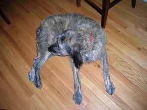
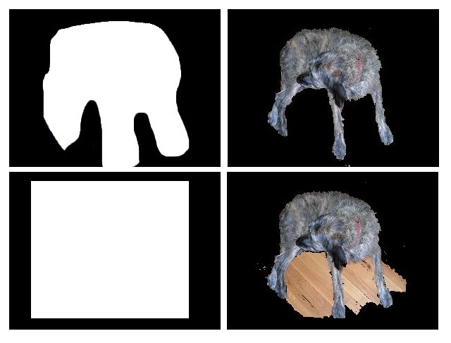
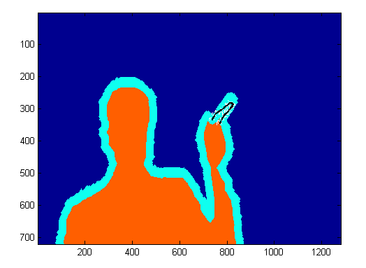
Jed Chou and Anna Weigandt The image segmentation problem is the following: given an image, a vector of pixels each with three associated red, green, and blue (RGB) values, determine which pixels should belong to the background and which should belong to the foreground. For example, in the following picture, the pixels which make up the dog should belong to the foreground, and the pixels making up the wood planks should belong to the background.
Summary
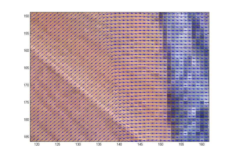
First we studied the grabCut algorithm and some general theory of image segmentation; we also played with some implementations of the grabCut algorithm to get a feel for how it worked. Anna wrote her own implementation of grabCut in matlab based on Gaussian Mixture Models which would take as input an image along with a manually-drawn matte and spit out a segmentation of the image into foreground and background. Our first goal was to get a clean segmentation of the dog picture shown above. Over the weeks we experimented with the dog picture by adjusting the algorithm parameters and we also discussed ways to extract more information from the color data to enhance the performance of Anna’s implementation. We added several matlab functions to do this. In the dog picture above, the problem mostly seemed to be that cutting along the long, upside-down U-shape between the dog’s hind legs and front legs was more expensive than cutting along the shorter distance spanned by a straight line from the bottom of the hind legs to the bottom of the front legs. We suspected that we needed to make it easier to cut along the this upside-down U-shape by decreasing the neighborhood weights along that arc. However, it wasn’t enough to just manually adjust the neighborhood weights–we wanted a way to automatically adjust the neighborhood weights so that such problems wouldn’t occur for other images. So our problem was to figure out which neighborhood weights to adjust and how to adjust them. First we tried using the directionality of the color data. The intuition was that if the colors in a subset of the image were running along a particular direction, then there should be an edge along that direction in the subset of pixels. We tried to capture the directionality in the color data by calculating the covariance matrix over small square windows of the image (the variance-covariance matrix of the variables X and Y where X was a vector consisting of the differences in color intensity in the horizontal direction and Y was a vector consisting of the differences in color intensity in the vertical direction). We then computed the spectrum of the covariance matrix centered at each pixel in the image. If the absolute value of the largest eigenvalue of the matrix was much greater than the absolute value of the smaller eigenvalue (which indicates a strong directionality along the direction of the corresponding eigenvector in that particular window), and also the largest eigenvector was almost horizontal or almost vertical, then we would decrease the corresponding horizontal or vertical neighborhood weight proportionally to the ratio of the eigenvalues. In theory this would make it less expensive to cut along the edges in the image. To check if the code was picking up directionality properly, we placed a vector field over the image where the vector at a pixel p was the eigenvector of the largest eigenvalue of the covariance matrix centered at p. Though the vector field seemed to capture the directionality properly, tweaking the edge weights in this way seemed to have little effect on the output of the algorithm: the large piece of wood flooring between the dog’s legs was still being categorized as foreground, even after we greatly magnified the adjustments to the edge weights based on the ratio of eigenvalues.
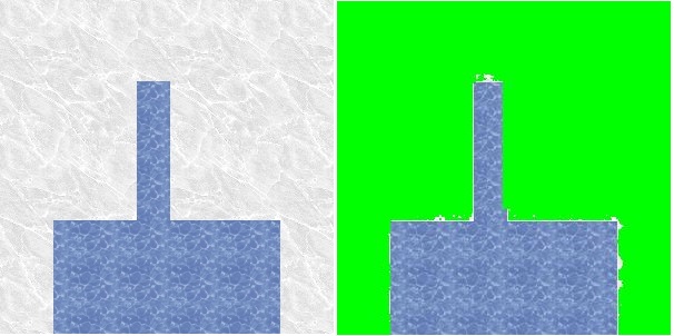
We next experimented with modifiying select node and neighborhood weights on the finger image. We manually marked certain pixels of the finger of the test image and adjusted the weights so that the selected pixels were forced into the foreground. This strategy only ensured the selected pixels were placed in the foreground. It failed to pull the rest of the finger into the foreground.
“how I spent this summer”
The summer was busy for PI4 students – whether those who just participated in the Computational Bootcamp (where a lot was learned, we hear), or those who worked in the research teams with Profs. Bronski and Deville (the “Train” phase of our program).
Below are links to their reports, dealing with
- Kuramoto model: Burson, Golze, Sisneros-Thiry; Ferguson, Terry, Gramcko-Tursi; Livesay, Ford, Gartland .
- Graph Laplacians: Burson, Livesay, Terry; Ferguson, Ford, Golze; Sisneros-Thiry, Gramcko-Tursi, Gartland.
- or Markovopoly: Gartland, Burson, Ferguson; Sisneros-Thiry, Ford, Terry.
Summer reports: working with applied mathematicians on real life problems
Several of our interns spent the summer working on various mathematical models stemming from real life challenges: understanding stability in power networks in their postmodern complexity; disentangling the intricacies of online search on two lines and understanding the limb development.
Below are their reports:
Nicholas Kosar, supervised by Alejandro Dominguez-Garcia;
Argen West, supervised by Prof. Zharnitsky;
Daniel Carmody and Elizabeth Field, supervised by Prof. Rapti;
Ben Fulan, supervised by Prof. Ferguson.
summer reports: shaping the canopy
PI4 Interns Nuoya Wang and Matthew Ellis spent this summer doing research under direction of Dr. Lebauer, a Research Scientist at Photosynthesis and Athmospheric Change Lab of UofI’s Energy Biosciences Institute. Below is their report.
This summer we focused on building a sugarcane canopy model and investigating into the direct sunlight photosynthesis effect.
The first task is how to extract features from a 3D image of one canopy. The data format is triangular mesh, which means the leaves and stems are divided into little triangles. This gives us a clue that we may use neighborhood relationship to define the structure of the canopy.
Firstly, it is easy to find the height of the canopy. We just need to find the points with largest z-coordinate and smallest z-coordinate then the difference is the height. So the main task is to extract leaf length, leaf width and leaf curvature.
To obtain features of a leaf, we need to divide a plant into different leaves and analyze each leaf. Since the plant is represented by a triangular mesh, we can interpret it into a graph. That is, we find unique vertices and construct the adjacency matrix. For example, if there are 10,000 unique points, our adjacency matrix will be a 10,000×10,000 one and if 10, 100, 1000 form a triangle, then the (10, 100), (100, 10), (10, 1000), (1000, 10), (100, 1000), (1000, 100) elements in matrix will be marked as 1.
We can use connected components algorithm, say, Bellman-Ford algorithm to split the graph into isolated components. In our sample data, it is more direct to do this because each leaf is not really “attached” to the stem which means stem is isolated from leaves. If the data is from reconstruction of real world data, we need to clean the data first, for example, we can calculate the number of neighbors for each vertex and delete some vertices with few neighbors. In this way some attached points will be separated. In the following figure 1, we have marked different components by different colors.
Since we have got one leaf from previous step, we can start to analyze it. The algorithm we use is Minimum Spanning Tree Algorithm.
In our problem we choose “weight” as the Euclidean distance between different points. After applying minimum spanning tree algorithm some of the unimportant connections are ignored and result is in figure 2:
Left: Figure 1; Right: Figure 2.
It is clear in figure 2 that the path which connect 2 red points can be used to estimate leaf length. So we used shortest path algorithm to find the path and calculate the path length. The 2 red points are defined as the pair with longest Euclidean distance. Leaf width can also be calculated from this minimum spanning tree. My algorithm is checking all points on the shortest path which connects the 2 red points, find 2 closest neighbors and leaf width at that point is defined as the sum of distance from the 2 neighbors. Finally, we choose the largest width as the width for whole leaf. Once we have the Euclidean distance of the 2 red points and the length of path connecting them, we can easily find the leaf curvature.
The second task in the summer project is to discuss the photosynthesis effect. We only considered the effect of direct sunlight. Our goal is to find the relationship between sunlit area ratio and height. The canopy model we used is still the triangular mesh model we have mentioned above.
In this part we focus on all vertices and introduce randomness into our algorithm. The basic principle for the algorithm is very simple: first we group all triangles’ vertices according to their heights. Second step is randomly choosing some points in one layer (that is, one group) to check if those points are shaded by higher level points or not. For example, if there are 1000 points in that group in total and we choose 200 of them. After calculation there are 100 points being shaded, then we assume there are 500 points being shaded in the original group. Using this simple sampling method, we can improve the efficiency of our algorithm by a lot.
Following are the results for direct sunlit ratios. In figure 3, x-axis is the height and y-axis is the ratio of shaded area. We tried several sunlight angles and got different results.
Figures 3 and 4 show the results. In figure 3, the azimuth angles for 3 pictures are 30, 60 and 90 degrees. Black lines are elevation=30 results, blue lines are for elevation=60 and red lines are for elevation=90. In figure 4, elevation angles for 3 pictures are 30, 60 and 90 degrees. Magneta lines are azimuth=0 results while black lines are azimuth=30 results, blue lines are for azimuth=60 and red lines are for azimuth =90.
internships: Ferguson’s lab
Ben Fulan worked on this project at Andrew Ferguson’s lab.
Here’s Ben’s final report.
This project arose out of the search for a vaccine to combat HIV and the obstacles faced by this search. While it is possible to create a vaccine that induces an immune response against the virus, the effectiveness of this approach is limited by the ability of the virus to mutate into strains which would no longer be targeted by the immune response. The goal of this project is to produce an immune targeting scheme that can do the most damage to the virus while taking into account its ability to mutate.
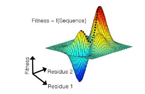
To this end, a measure of the fitness of the virus is needed. This takes the form of a fitness landscape, which gives the virus’s ability to replicate as a function of its amino acid sequence. (See figure below – the dashed line indicates a mutation path from a potentially immune-targeted global maximum to a local maximum.) In particular, this amino acid sequence can be described using a binary string, where 0 represents the natural (“wild type”) form of the amino acid and 1 represents a mutant. The fitness function can then be constructed from empirical data. This function assigns a fitness cost to each mutation and also contains terms to represent interactions between pairs of mutations, which can be either beneficial or harmful.
Once we have obtained the fitness function, we can add a term representing immune pressure that, for each amino acid, imposes a penalty for not mutating, effectively forcing the virus to mutate into a lower-fitness state. This modified function measures the viral fitness given a particular amino acid sequence; the next step is to produce a function that measures the overall fitness of the virus across all possible states. This function should give more weight to high-fitness states, since it is more likely that the virus will be found in such a state. One such function is
\[
\sum_z \exp{−\beta E(z,b)},
\]
where \(E\) is a version of the fitness function described above (in this case low energy corresponds to high fitness), \(z\) is the binary amino acid sequence, \(b\) is the sequence representing immune pressure, and the “inverse temperature” \(\beta\) represents the difficulty of mutation. Finally, we can cast the problem as an optimization problem as follows: minimize the overall fitness function subject to constraints on b (since only so much immune pressure can be applied). We then develop an algorithm to perform this optimization and obtain an optimum immune pressure sequence \(b\).
We can then check these results against empirical data; if the data match poorly, we can reconsider our choice of the overall fitness function.
internships: at John Deere
We will start a series of posts about the topics our interns are working on. We start with Sishen Zhou and Han Wang, who are working this summer at John Deere, dealing with
Data Analysis for High Precision Agriculture
Maps of yield distribution are crucial for precision agriculture. A yield map with high resolution can help farmers precisely perform future agricultural operations, such as applying fertilizer and planting seeds according to geographic data.
The problem we are working on at John Deere is to find a way to determine the response function of a combine harvester that mixes plants during the harvest operation.

To be more precise, the crop cut from the field takes a while and multiple paths within the combine from cutting to measurement at the crop yield monitor. This delay and mixing is captured in a response function, and the readings of the yield monitor is approximately a convolution of the real yield distribution with the response function. So once we find the response function, we will be able to create a much more accurate map of yield distribution with deconvolution algorithms.
The following figure illustrates a response function and the delay caused by it at the yield monitor readings.
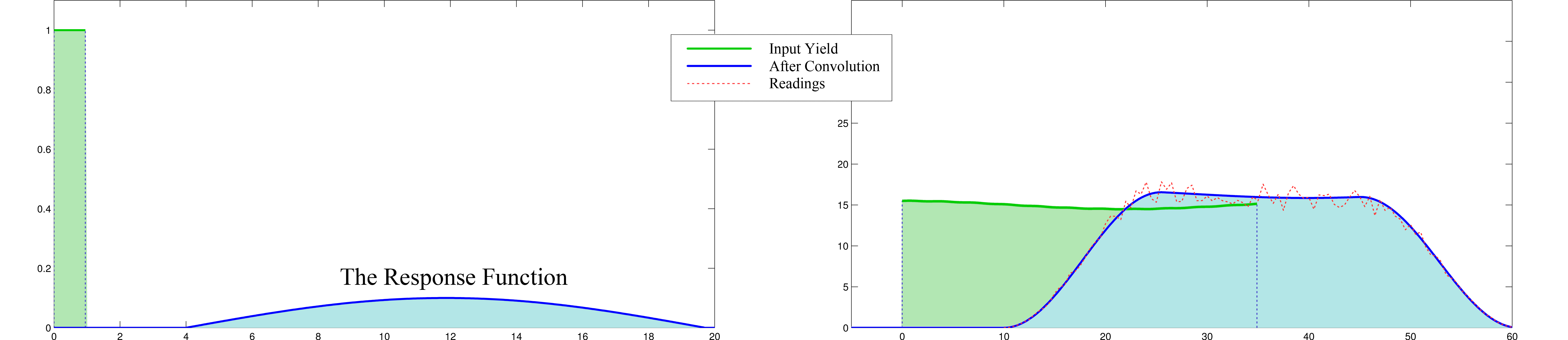
This problem is not trivial since the yield is processed within the combine in several complicated steps. The combine has to be treated as a black box causing the delay.
We are now proposing two methods to address the problem. The first one is the classic blind deconvolution approach developed in image and signal processing problems. The other one is to apply Fourier transformation on the data to recognize the frequency information of the response. In the second method, a parametric model may have to be assumed for the response function.
summer 2014
PI4-PREPARE programs
- Computational Mathematics Bootcamp, led by Prof. Anil Hirani, and Sean Shahkarami (TA)
Dates: June 9-20, in 239 Altgeld Hall
Two week intensive session on computation in a scientific environment.
See the Bootcamp homepage. - Deterministic and Stochastic Dynamics of a Social Network, led by Prof. Jared Bronski
Dates: June 2-6 and June 23-July 25, in 159 Altgeld Hall
Social interaction networks are an important part of the human experience, whether it is relations among subtribes of the Gahuku-Gama people of the highlands of New Guinea or between the 1.1 billion users of Facebook. We will use analysis and numerics to explore several models of deterministic and stochastic dynamics on a network, including a gradient flow model intended to explain social balance theory (“The enemy of my enemy is my friend”) and the Kuramoto model, a model governing synchronization of oscillations, from the flashing of fireflies to the synchronization of electrical generators. - Modeling and Analysis of Mathematical Challenges in Biology led by Prof. Lee DeVille
Dates: June 2-6 in 173 Altgeld Hall, and June 23-25, July 1-2 in 123 Altgeld Hall computer lab.
More information coming soon!
PI4-TRAIN programs
Illinois Biomath program – students can be attached to one of the existing summer Biomathematics programs, and can also participate in the Computational Mathematics Bootcamp. Topics in Summer 2014 will include:
- disease dynamics and evolution of host-resistance and pathogen-virulence,
- the visual system of fish,
- ants and networks, in particular how they construct colonies.
Dates depend on host and student schedules. Students can participate also in the Computational Mathematics Bootcamp.
PI4-INTERN topics
Industrial internships: at Personify, John Deere, Caterpillar, and possibly more.
Scientific internships:
- Molecular dynamics simulations of biophysical systems (e.g., peptides, lipids) and scientific data analysis and modeling using nonlinear machine learning and/or Bayesian inference model building.
- Synchronization and control of small-footprint power systems.
- Mechanisms responsible for shaping the patterns of morphological (i.e., form and structure) evolution that characterize the history of life.
- This project will seek to understand the three-way relationship among complexity increases in biological systems, information flow between scales in such systems, and thermodynamics. The intern will contribute to this understanding by modeling ecological dynamics over multiple time scales, through analytical work and computer simulation.
Internship dates depend on host and student schedules.
scientific computing best practices
Mathematicians tend to view their work as somewhat Bohemian endeavor, driven by inspiration and imagination and not by process or organization. At the same time, the research enterprise in sciences and engineering is far more often perceived as a structured team effort, thoroughly documented, perspirational rather than inspirational.
This comparison is true only to some degree – perhaps less than we use to think: our discipline depends on a rigorous (one might say, tedious) process of verification and social acceptance of a result, we work increasingly often in teams, and schedule our research efforts around our teaching or travel engagements… With all the differences, mathematical research is not as far from the general research practices as we might believe.
Still, to someone trained in mathematics, experiencing the daily practices of a scientific or engineering lab might feel a cultural shock. A well run lab operates as a machine, with lots of rules and practices woven into the daily routine.
The good news is that these rules, by and large, make a lot of sense. They eliminate (a fraction of) noise, waste and confusion, and open room for creativity and imagination. Learning and adopting them make life easier, and research better.
Below are some of the best practices relevant to PI4 where most of the internships will deal in some degree with scientific computing. They are borrowed from a PLoS article Best Practices for Scientific Computing (thanks to David L. for pointing it to me).
Summary of Best Practices
- Write programs for people, not computers.
- A program should not require its readers to hold more than a handful of facts in memory at once.
- Make names consistent, distinctive, and meaningful.
- Make code style and formatting consistent.
- Let the computer do the work.
- Make the computer repeat tasks.
- Save recent commands in a file for re-use.
- Use a build tool to automate workflows.
- Make incremental changes.
- Work in small steps with frequent feedback and course correction.
- Use a version control system.
- Put everything that has been created manually in version control.
- Don’t repeat yourself (or others).
- Every piece of data must have a single authoritative representation in the system.
- Modularize code rather than copying and pasting.
- Re-use code instead of rewriting it.
- Plan for mistakes.
- Add assertions to programs to check their operation.
- Use an off-the-shelf unit testing library.
- Turn bugs into test cases.
- Use a symbolic debugger.
- Optimize software only after it works correctly.
- Use a profiler to identify bottlenecks.
- Write code in the highest-level language possible.
- Document design and purpose, not mechanics.
- Document interfaces and reasons, not implementations.
- Refactor code in preference to explaining how it works.
- Embed the documentation for a piece of software in that software.
- Collaborate.
- Use pre-merge code reviews.
- Use pair programming when bringing someone new up to speed and when tackling particularly tricky problems.
- Use an issue tracking tool.
Computational Mathematics Bootcamp
To help our Mathematics students to acquire – as quickly and as painlessly as possible – the basic computational skills expected in scientific and engineering research labs, PI4 has run a 2-week long Computational Mathematics Bootcamp for Graduate Students.
We hope not only to quickly raise the basic computational literacy of PI4 members to the levels expected by their potential internship hosts, but, perhaps as important, to impart the culture of best practices of scientific and engineering computing.
The camp is open to all students confirmed with PI4, whether funded or not.
Materials for download
Computational Bootcamp 2019 (9 days on Python, R and data science)
Computational Bootcamp 2018 – Part 1 (6 days on data science)
Computational Bootcamp 2018 – Part 2 (3 days on Mathematica fundamentals)
Computational Bootcamp 2017 (10 days, focus on data science)
Computational Bootcamp 2016 (10 days, focus on scientific computing)
Computational Bootcamp 2015
Linear Algebra Workshop 2019 (3 days)